Search-
Search
a tool for problem solving of AI applications.
Typical problem includes:
finding the solution to a puzzle e.g. the 8-puzzle
finding a proof for a theorem in logic or mathematics
finding the shortest path connecting a set of non-equidistant points (the TSP traveling salesman problem)
finding a
sequence of moves that will win a game, or the best move to make at
a given point in a game.
[Note that one cannot explore all
possible moves until end games, unless the game is simple, such as
tic-tac-toe.]
finding a
sequence of transformations that will solve a symbolic integration
problem.
Problem Representation
State space representation
problem reduction representation
game tree
search method
blind state-space search
blind AND/OR graph search
heuristic state-space search (A*)
heuristic search of an AND/OR graph
game tree search
Components of Search Systems
problem solving systems can be described in terms of 3 main components:
A Database
describes both the current task domain situation and the goal
consists of
variety of different kinds of data structures
e.g. arrays, lists,
sets of predicates calculus expressions, property lists, semantic
networks, ...
In Chess playing:
current situation - chess board configurations
goal - a winning board configuration
In theorem proving:
current situation - assertions representing axioms, lemmas and theorem already proved.
goal - assertion representing the theorem to be proved.
In information retrieval application
current situation - a set of facts
goal - query to be answered
In robot problem solving
current situation - a world model consisting of statements describing the physical surroundings of the robot
goal - a description that is to be made true by a sequence of robot actions
A Set of Operators
used to manipulate the database
In chess, rules for moving chessman
In theorem proving, rules of inference such as modus ponens and resolution.
In symbolic integration, rules for simplifying the form to be integrated (e.g. integration by parts)
A Control Strategy
decide what to
do next
e.g. what operator to apply and where to apply
Note that the choice of control strategy affects the contents and organization of the database.
The objectives: to achieve the goal by applying an appropriate sequence of operators to an initial task domain situation.
each application of the operator modifies the situation
representation will maintain data structures showing the effects of each alternative sequence.
control strategy investigate (search) various operator sequences in parallel that looks "promising".
[If description of
task domain is too large, multiple version cannot be stored, and
backtracking may be required.]
Reasoning forward & backward
Reasoning forward
application of operators to produce a modified situation, forward from its initial configuration to one satisfying a goal situation.
for example, robot will start from current location and explore forwards.
said to be data driven or bottom-up. (The goal is at the top)
Reasoning backward

the goal statement is converted to one or more sub-goals that are (hopefully) easier to solve and whose solutions are sufficient to solve the original problem, e.g.
said to be goal-directed or top-down.
much human problem-solving behaviour is observed to involve reasoning backwards. (Many AI programs are based on this strategy).
Can combine forward and backward reasoning.
Graph Representation
tree structure is commonly used. the nodes (states) are connected together. The descendent of a node is the nodes (states) that can be reached from the current node.
In general, graph structure is needed, because you may have repeated states.
for problem reduction, a node can be solved only if ALL of its sub-problem can be solved. (e.g. integration by parts will require all parts to be integrated.).
Use AND/OR graph.
Game Tree representation for game playing involving two opponents. Each player will try to maximize his own advantage.
Many problem have infinite search space, or unimaginably large search space (e.g. chess, go etc), and cannot search the entire space. Must stop and do an estimation on the goodness of the node at some time.
Need to expand the node when required, cannot store the entire search space.
Have to limit the search - exhaustive search is rarely feasible in non-trivial problems (combinatorial explosion)
Use of heuristic knowledge from the problem domain to help focus the search.
State spaces Representation of Problems
state spaces are spaces of states [!]
each situation (or configurations) is represented by a state, usually in the form of node of a graph.
there is an initial state and final state representing the initial and final configuration. (e.g. in chess playing, the initial state is just the startup board configuration, while the final state is any winning configuration)
arcs exists from node A to node B if you can move within 1 step from configuration A to configuration B.
objective: to
find a path from the initial state to a final state, usually via
searching.
Example:
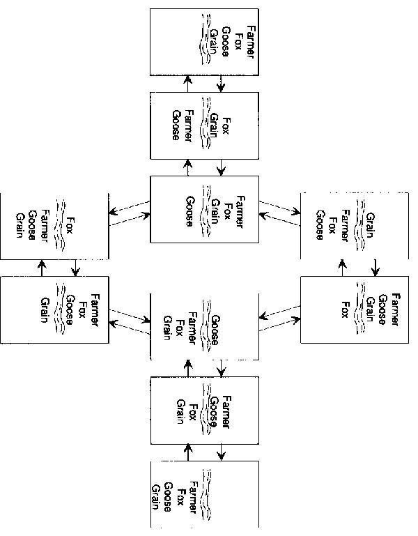
(farmer, fox, goose and grain)
A farmer wants to move himself, a
silver fox, a fat goose and some tasty grain across a river.
Unfortunately, his goat is so tiny he can take only one of his
possessions across on any trip. Worse yet, an unattended fox will
eat a goose, and an unattended goose will eat grain, so the farmer
must not leave the fox alone with the goose or the goose alone with
the grain. What is he to do?
each state can be represented by a 4-tuple, e.g. [L R L R], representing the location of framer, fox, goose and grain respectively. L 0 left side of river, R 0 right side of river.
initial state: [L L L L], final state: [R R R R]
Some state are not allowed by problem description, e.g. [L L R R], where the goose and grain are on the same side of the river.
Also, not all nodes are connected by arcs, because the boat must be operated by the farmer, and the above rule also applies on the boat.

Example: (8-puzzle)
|
2 |
1 |
6 |
|---|---|---|
|
4 |
|
8 |
|
7 |
5 |
3 |
Initial
Configuration
|
1 |
2 |
3 |
|---|---|---|
|
8 |
|
4 |
|
7 |
6 |
5 |
Solution Configuration
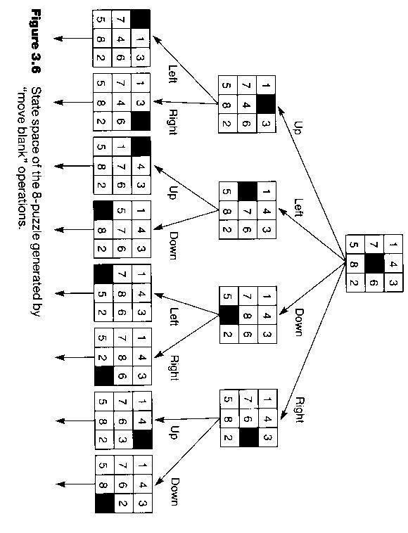
A tile may be moved by sliding it vertically or horizontally into an empty square.
state: represented by a 3x3 matrix as above.
Operators: instead of sliding the tile, represented as moving the empty square: UP, DOWN, LEFT, RIGHT.
there are a total of 181,440 possible states.
a common variation of state-space problem require finding not just any path but one of minimum cost between an initial node and a goal node. e.g. Traveling Salesman Problem

Sometimes the state-space graph is too large to be represented explicitly. The problem becomes generating just enough of the graph to contain the desired solution paths.
Problem Reduction Representation
consists of 3 parts
initail problem description
a set of operators for transforming problems to sub-problems
a set of primitive descriptions (whose solution is immediate)
Reasoning proceeds backwards from the initial goal.
Example: (Tower of Hanoi)

only 1
operator:
Given distinct pegs i, j and k, moving a stack of size
n>1 from peg i to peg k can be replaced by the 3 sub-problems:
moving a stack of size n-1 from i to j
moving a stack of size 1 from i to k
moving a stack of size n-1 from j to k
primitive problem:
moving a single disk from one peg to another, provided that no smaller disk is on the receiving peg. Otherwise problem unsolvable.
AND/OR Graph
Each node
represents either a single problem or a set of problems to be
solved.
The start node correspond to the original problem
a node representing a primitive problem, called a terminal node, has no descendants
P is reduced to sub-problem set A, B, C
if P can be solved if any one of sets A, B, or C can be solved, A, B, C are called OR nodes.
if P can be solved only if all its members can be solved, they are called AND nodes.
the arcs leading to AND-node successors of a common parent are joined by a horizontal line.

Example: (robot planning)


A node is solvable if
it is a terminal node (a primitive problem)
it is a non-terminal node whose successors are AND nodes that are all solvable, or
it is a non-terminal node whose successors are OR nodes and at least one of them is solvable.
Game Tree
a representation of all possible plays of a game.
root node 0 initial state (the 1st player's turn to move)
successors 0 states he can reach in one move
their successors are the other player's possible reply.
terminal node 0 configuration representing win, loss or draw
each path from the root node to a terminal node gives a different complete play of the game.

Example (tic-tac-toe)
Search Strategies
Blind State-Space Search
do not use any domain specific information to assist the search.
Assumption made:
there is a procedure called expand for finding all successors of a given node.
the state space is a tree (can convert a graph into a tree with repeated nodes)
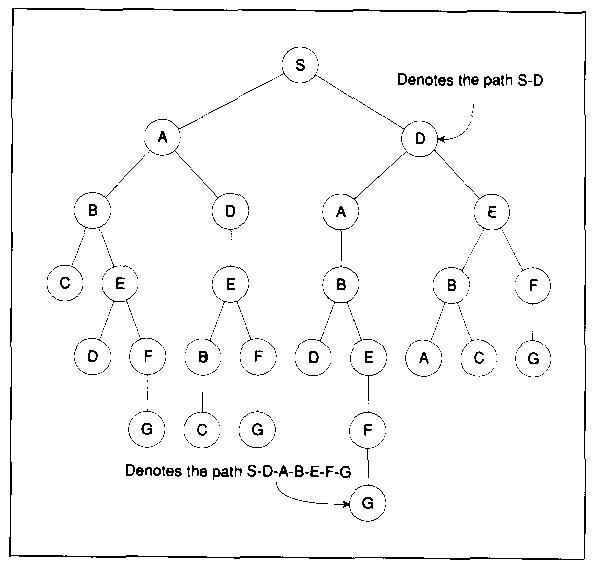

Breadth-first search
expand nodes in order of their proximity to the start node, measured by the no. of arcs between them.
Algorithms:
Put the start node on a list, called OPEN, of unexpanded nodes. If the start node is a goal node, a solution is found.
If OPEN is empty, no solution exists
Remove the first node, n, from OPEN and place it in a list, called CLOSED, of expanded nodes
Expand node n. If it has no successors, goto 2.
Place all successors of node n at the end of the OPEN list.
If any of the successors of node n is a goal node, a solution has been found. Otherwise goto 2.
2. Depth-first search
characterized
by the expansion of the most recently generated, or deepest
node first, where the depth of a node is defined as:
start
node: depth 0
other nodes: depth of its predecessor + 1
note that in many problems, the state-space tree may be of infinite depth. A maximum is often placed on the depth of nodes to be expanded.
Algorithms
Put the start node on a list, OPEN, of unexpanded nodes. If it is a goal node, a solution has been found.
If OPEN is empty, no solution exists.
Move the first node, n, on OPEN to a list, CLOSED of expanded nodes.
If the depth of node n is equal to the max depth, goto 2.
Expand node n. If it has no successor, goto 2.
Place all successors of node n at the beginning of OPEN.
If any of the successors of node n is a goal node, a solution has been found. Otherwise, goto 2.
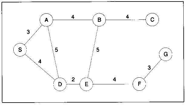


 Example:
Traces of searches:
Breadth-first search:
open=[S]; closed=[]
open=[A,D]; closed=[S]
open=[D,B,D]; closed=[S,A]
open=[B,D,A,E]; closed=[S,A,D]
open=[D,A,E,C,E]; closed=[S,A,D,B]
...
Depth-first search:
open=[S]; closed=[]
open=[A,D]; closed=[S]
open=[B,D,D]; closed=[S,A]
open=[C,E,D,D]; closed=[S,A,B]
open=[E,D,D]; closed=[S,A,B,C]
open=[D,F,D,D]; closed=[S,A,B,C,E]
...
8-puzzle:
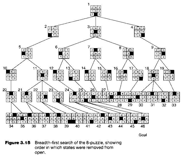
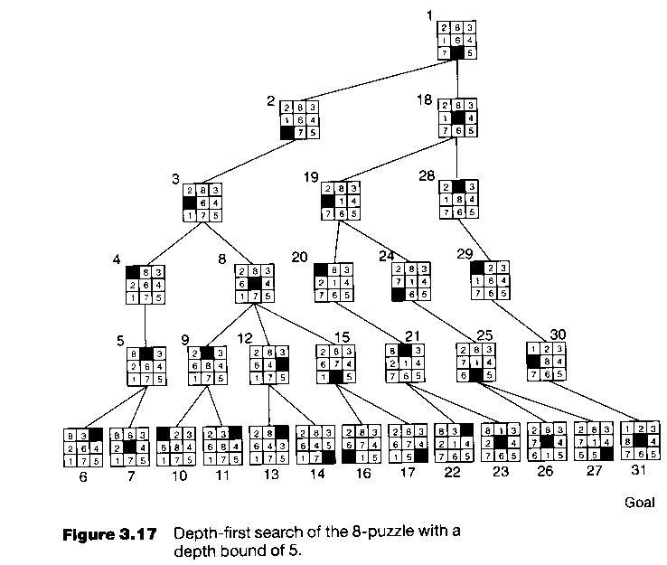
Uniform-cost Search
generalized to find the cheapest path from the start node to the goal node.
A non-negative cost is associated with every arc joining two nodes. Cost of solution path=sum of arc costs along the path.
if all arcs have equal cost 0 breadth-first search
Let c(i,j) = cost of arc from node i to node j.
g(i) = cost of a path from start node to node i
Algorithm:
Put the start node S on a list called OPEN, of unexpanded nodes. If the start node is a goal node, a solution has been found. Otherwise, set g(s)=0.
If OPEN is empty, no solution exists.
Select from OPEN a node i such that g(i) is minimum. If several nodes qualify, choose node i to be a goal node if there is one; otherwise, choose among them arbitrarily. Move node i from OPEN to a list CLOSED of expanded nodes.
If node i is a goal node, a solution has been found.
Expand node i. If there is no successor, goto 2.
For each
successor node j of node i, compute
g(j) = g(i) + c(i,j)
and
place all successor nodes j in OPEN.
Goto 2.
Search
Result
(value of g(x) is in parenthesis)
OPEN=[S(0)]; CLOSED=[]
OPEN=[A(3), D(4)]; CLOSED=[S]
OPEN=[B(7), D(8), D(4)]; CLOSED=[S,A]
OPEN=[B(7), D(8), A(9), E(6)]; CLOSED=[S,A,D]
OPEN=[B(7), D(8), A(9), B(11), F(10)]; CLOSED=[S,A,D,E]
...
Bi-directional Search
search is likely to grow exponentially with the no. of search levels.
Combine forward and backward search. Replace a single search graph by two smaller graphs (the number of level will be halved), one starting from start node, the other from goal node.
Search will terminate when two graphs intersect.
Empirical studies show that bi-directional search expands only ~1/4 as many nodes as uni-directional search.
Only applicable if we can expand backwards.
Notations:
s=start node, t=goal node.
S-OPEN and S-CLOSED are lists of unexpanded and expanded nodes respectively, generated from start node.
T-OPEN and T-CLOSED are lists of unexpanded and exapned nodes, respectively, generated from goal node.
cost from node n to node x: c(n,x)
gs(x) = shortest path so far from s to x
gt(x) = shortest path so far from x to t
Algorithm:
Put s in
S-CLOSED, with gs(s)=0. Expand node s. For each successor node x,
place x on S-OPEN and set gs(x) to c(s,x).
Correspondingly, put t
in T-CLOSED with gt(t)=0. Expand node t. For each predecessor
node x, place x in T-OPEN and set gt(x) to c(x,t).
Decide whether
to go forward or backward, e.g. (1) alternate between forward &
backward, or (2) move backward if T-OPEN contains fewer nodes than
S-OPEN, otherwise forward.
If forward, goto (3), else goto (4).
Select from S-OPEN a node n at which gs(n) is minimum. Move n to S-CLOSED. If n is also in T-CLOSED, goto (5). Otherwise, for each successor x of n:
If x is on neither S-OPEN nor S-CLOSED, then add x to S-OPEN. gs(x) = gs(n) + c(n,x)
If x was already on S-OPEN, a shorter path to x may have just been found. Compare the previous cost gs(x) with gs(n)+c(n,x). If the latter is smaller, set gs(x) to the new path cost.
If x was already on S-CLOSED, do nothing (even though a new path to x has been found, its cost must be at least as great as the cost of the path already known)
Return to (2).
Select from T-OPEN a node at which gt(n) is min. Move n to T-CLOSED. If n is also in S-CLOSED, goto (5). Otherwise, for each predecessor x of n:
If x is on neither T-OPEN nor T-CLOSED, then add it to T-OPEN. Set gt(x) = gt(n) + c(x,n)
If x was already on T-OPEN and a shorter path from x to t has just been found, set gt(x) to the new value.
If x was already in T-CLOSED, do nothing.
Return to (2).
Consider the set of nodes that are in both S-CLOSED and either T-CLOSED or T-OPEN. Select from this set a node n for which gs(n)+gt(n) is minimum.
Non-deterministic Search
Expand a node chosen at random.
Algorithm:
Put the start node s on a list called OPEN of unexpanded nodes. If the start node is a goal node, a solution has been found.
If OPEN is empty, no solution exists
Remove the first node n from OPEN and place it in a list, called CLOSED, of expanded nodes.
Expand node n. If it has no successors, goto 2.
Place all successors of node n at random places in the OPEN list.
If any of the successors of node n is a goal node, a solution has been found. Otherwise, goto 2.
Blind AND/OR Graph Search
Assumptions:
the search space is an AND/OR tree and not a general graph.
when a problem is transformed to a set of sub-problems, the sub-problems may be solved in any order.
Breadth-first search
Put the start node on a list OPEN of unexpanded nodes.
Remove the first node n from OPEN.
Expand node n, generating all its immediate successor, and for each successor m, if m represents a set of more than one sub-problem, generate successors of m corresponding to the individual sub-problems. Attached to each newly generated node, a pointer back to its immediate predecessor. Place all the new nodes that do not yet have descendants at the end of OPEN.
If no successors were generated in (3), then
label node n solvable
If the unsolvability of n makes any of its ancestors unsolvable, label these unsolvable.
If the start node is labeled unsolvable, exit
remove from OPEN any nodes with an unsolvable ancestors.
Otherwise, if any terminal nodes were generated in (3),
label these nodes solved.
if the solution of these terminal nodes makes any of their ancestors solved, label them solved.
if start node is labeled solved, exit
remove from OPEN any nodes that are labeled solved, or that have a solved ancestor.
Goto 2.
Depth-first search
by chaning step (3) of previous algorithm:
if the depth of n is less than the depth bound, then expand node n, generating all its immediate successors and for each successor m, if m represents a set of more than one sub-problem, generating successors of m corresponding to the individual sub-problems. Attach to each newly generated node, a pointer back to its immediate predecessor. Place all the new nodes that do not yet has descendants at the beginning of OPEN.
Example:

Breadth-first search:
|
OPEN |
unsolable |
Solvable |
|---|---|---|
|
[S] |
|
|
|
[A] |
|
|
|
[B,C,D] |
|
|
|
[C,D,E] |
|
|
|
[D,E,F] |
|
|
|
[E,F] |
D |
|
|
[F] |
D,E,B |
|
|
[G,I] |
D,E,B |
K |
|
[I] |
D,E,B |
K,J,G |
|
[] |
D,E,B |
K,J,G,L,I,H,F, |
Depth-first search:
|
OPEN |
unsolvable |
Solvable |
|---|---|---|
|
[S] |
|
|
|
[A] |
|
|
|
[B, C, D] |
|
|
|
[C, D] |
E |
|
|
[F D] |
E |
|
|
[G, I D] |
E |
K |
|
[I D] |
E |
K,J,G |
|
[D] |
E |
K,J,G,L,I,H |