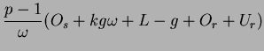
We first derived the lower bound cost for the complete exchange operation
on our abstract model - the completely connected cluster. Assuming
that each node is capable to send and receive a message in one time
unit, such that
![]() .
With this capability, a process can actively send and receive at the
same time, thus can fully utilize the communication network. In this
study, we are only focusing on the communication performance in exchanging
large data block, which is the general scenario happened in most scientific
and numerical computations on message passing machines. To simplify
the analysis, we assume that each data block corresponds to k
data packets. Therefore, the minimum amount of packets being sent
and received in the complete exchange operation per process is
.
With this capability, a process can actively send and receive at the
same time, thus can fully utilize the communication network. In this
study, we are only focusing on the communication performance in exchanging
large data block, which is the general scenario happened in most scientific
and numerical computations on message passing machines. To simplify
the analysis, we assume that each data block corresponds to k
data packets. Therefore, the minimum amount of packets being sent
and received in the complete exchange operation per process is ![]() packets or
packets or ![]() bytes if each data packet is of size b
bytes.
bytes if each data packet is of size b
bytes.
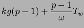
As the minimal time in sending or receiving a packet of size b bytes
is bounded by the send gap (![]() ) and receive gap (
) and receive gap (![]() ),
and each machine can inject or receive no more than one packet within
this gap. Therefore, we deduce that the minimal time required for
the complete exchange operation under such a cluster communication
abstraction is
),
and each machine can inject or receive no more than one packet within
this gap. Therefore, we deduce that the minimal time required for
the complete exchange operation under such a cluster communication
abstraction is
Thus, any solution to the k-item complete exchange
operation on the cluster is optimal if it takes ![]() time
units to finish the operation. Carry on with the deduction, we see
that the necessary conditions to satisfy the above optimality are:
time
units to finish the operation. Carry on with the deduction, we see
that the necessary conditions to satisfy the above optimality are:
With the assumption of complete-connected topology, links and bandwidth are sufficient but contention still exists if message transmissions are not well scheduled. In particular, any efficient algorithm in realizing the complete exchange operation must balance between synchronization and contention. This is because, due to the distributed nature of the clusters, it is difficult to impose a lock-step schedule. As most of the synchronization operations are implemented by software means, this further impedes on normal data communication and contends for network resources. In the following subsections, we review the communication schedules used by different algorithms for the complete exchange operation, and use our performance model to evaluate their performance.
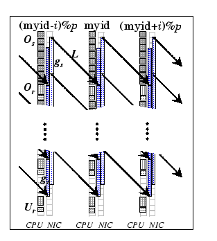
This algorithm is the simplest way to schedule communications without
node contention. It takes p-1 communication rounds, and during
each round, each process sends out k items to one partner,
and receives k items from another partner, which is determined
by a shift pattern.
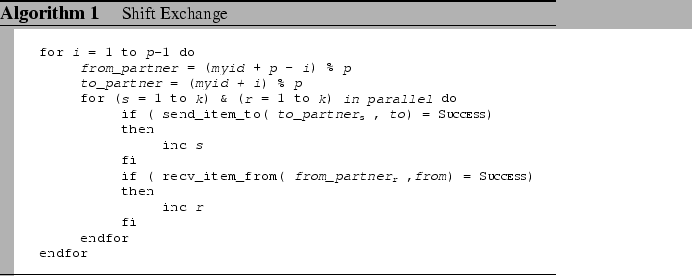
As depicted in Algorithm 1, during each round, each node uniquely maps to one sendto and recvfrom partners, thus exhibits no node contention. However, the non-stalling condition (Condition 2) is not enforced under this scheme. Although there is no explicit synchronization appeared between consecutive rounds and both send and receive operations are of non-blocking semantics, the p-1 rounds have an implicit synchronization cost that introduces bubbles to the network pipelines.
For example, Figure 5.1 depicts a typical communication round. Both the send and receive channels are idle until the first byte of the first packet is being injected into the network. Similarly, after receiving the last byte of the last packet, both channels are idle until the cluster node has finished handling the last packet of this round. The predicted communication cost for this complete exchange operation is
From the cost formula, we notice that this algorithm is not optimal
as there is a messaging overhead which is proportional to the number
of cluster nodes, as denoted by
![]() .
.
In the pairwise exchange algorithm, nodes are pairing up for direct
exchange in each round. Traditionally, the pairing pattern is based
on the Exclusive Or (XOR) binary operation. From high-level
prospective, the communication cost of the pairwise exchange algorithm
coincides with that of the shift exchange as both algorithms involve
the same number of communication rounds and communication load. Therefore,
we can consider that
![]() . We will discuss later
how they may be different from an implementation view, such that their
cost formulae may be different.
. We will discuss later
how they may be different from an implementation view, such that their
cost formulae may be different.
The major drawback of the XOR bitwise operation is the requirement
of ![]() in order to symmetrically pairing up all the nodes.
For the case with
in order to symmetrically pairing up all the nodes.
For the case with
![]() , the number of rounds becomes
, the number of rounds becomes
![]() , and during each round,
not all the nodes find a matching partner. The solution to the pairing
problem is to find an algorithm that matches our completely-connected
topology. The pairing problem can be formulated as an edge-coloring
problem on any connected graph. It is defined as:
, and during each round,
not all the nodes find a matching partner. The solution to the pairing
problem is to find an algorithm that matches our completely-connected
topology. The pairing problem can be formulated as an edge-coloring
problem on any connected graph. It is defined as:
Given a graph, with
nodes connected by a set of edges (E), what is the minimum number of colors needed to color the edges of G so that no two adjacent edges are assigned the same color.
In graph theory, this is also defined as the edge-chromatic index
![]() of G. Thus, the solution to our schedule problem
is to find an algorithm for edge-coloring the complete graph, with
the edge-chromatic index represents the number of communication rounds.
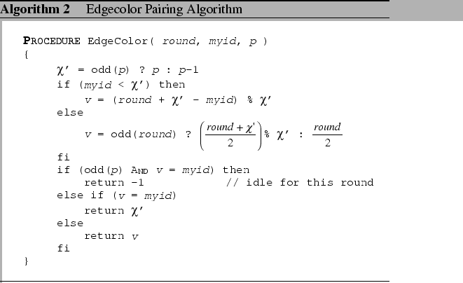
Due to its uniqueness, there exists a simple numerable solution comparable
to the XOR bitwise operation for
of G. Thus, the solution to our schedule problem
is to find an algorithm for edge-coloring the complete graph, with
the edge-chromatic index represents the number of communication rounds.
Due to its uniqueness, there exists a simple numerable solution comparable
to the XOR bitwise operation for ![]() , and is being
described and proved in [40]. By incorporated this
algorithm (Algorithm 2) to the pairwise exchange scheme,
we have the generalized pairwise exchange algorithm. Under this mapping
scheme, the performance is only slightly deteriorated with p
communication rounds for all odd cases, instead of having p-1
communication rounds for all even cases.
, and is being
described and proved in [40]. By incorporated this
algorithm (Algorithm 2) to the pairwise exchange scheme,
we have the generalized pairwise exchange algorithm. Under this mapping
scheme, the performance is only slightly deteriorated with p
communication rounds for all odd cases, instead of having p-1
communication rounds for all even cases.
The above two algorithms have a messaging overhead which is depended on the number of communication rounds. If k is small and p is large, they would perform poorly. A simple solution to this problem is by removal or reduction of this messaging overhead. We observe that the previous two schedules are arranged to avoid node contention at the message level, such that during the exchange, the whole message (k data packets) is being sent continually to the destination.
The synchronous shuffle schedule (Algorithm 3), effectively
multiplexes all the p-1 messages in a single round by applying
a contention-free schedule at the packet level without explicit synchronization
operation. Based on that packet-level scheduling, at a particular
instant ![]() (assume logically synchronized), each process
is sending its
(assume logically synchronized), each process
is sending its ![]() packet to the process
packet to the process ![]() directly.
And
directly.
And ![]() is derived from a node contention-free permutation
scheme (
is derived from a node contention-free permutation
scheme (![]() ), e.g. the shift pattern, the XOR
pattern or the edgecolor pattern. As each process can uniquely match
to different process at each packet transmission step, it guarantees
no two packets are directed to the same destination at the same instant,
thus no node contention. The predicted communication cost for this
complete exchange operation is
), e.g. the shift pattern, the XOR
pattern or the edgecolor pattern. As each process can uniquely match
to different process at each packet transmission step, it guarantees
no two packets are directed to the same destination at the same instant,
thus no node contention. The predicted communication cost for this
complete exchange operation is
From the cost formula, we notice that the messaging overhead is kept
constant, and is not depended on p or k. In addition,
this cost formula matches exactly to our optimal formula ![]() .
This shows that the scheme can effectively utilize the send and receive
channels by multiplexing all the messages seamlessly to a single pipeline
flow without unnecessary synchronization delay.
.
This shows that the scheme can effectively utilize the send and receive
channels by multiplexing all the messages seamlessly to a single pipeline
flow without unnecessary synchronization delay.
If every operation is executed on schedule, and the network resources
are scalable, then, the permutation scheme of the synchronous shuffle
exchange could be finished in minimal time. However, in reality, logical
synchronization is not enforced due to the distributed nature of the
cluster system. Random delays between communication events, such as
scheduling delays, could break this harmony and result in ``transient
hot-spot'' in the switch. Observed that the more packets are targeting
to the same output link, which are arriving from different sources
at different time period, the higher chance of having conflicts even
under a regular and uniform pattern. When two or more packets contend
for the same output link, buffering of conflicting packets would result
in routing delay. As the buffering technique within the switch has
an enormous impact on the network performance, we reckon that the
synchronous shuffle scheme could suffer on clusters with input-buffered
switches due to the head-of-line blocking problem.
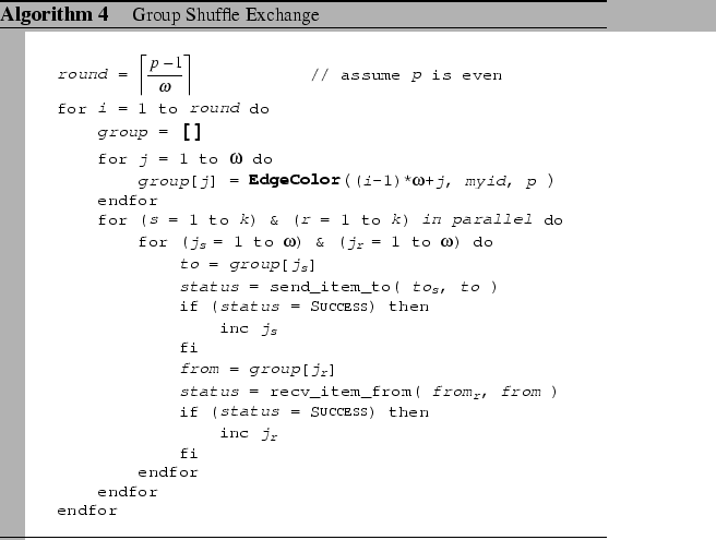
Group shuffle exchange (Algorithm 4) is a hybrid approach
that combines the pairwise exchange and the synchronous shuffle exchange
algorithms. The main idea is to overcome the HOL problem but still
achieving comparable performance as compared to the synchronous shuffle
scheme. In pure pairwise exchange scheme, packets appear in each input
port are destined to a unique outgoing port in each round, thus HOL
blocking does not exist even under input-buffered switch. However,
in the pairwise scheme, the startup overhead is linearly proportional
to the number of communication rounds, which hinders its efficiency.
For the group shuffle exchange, we reduce the number of communication
rounds to
![]() . In
each round, a processor is performing a synchronous shuffle exchange
with at most
. In
each round, a processor is performing a synchronous shuffle exchange
with at most ![]() partners. The main idea of this scheme
is to limit the degree of fan-out (
partners. The main idea of this scheme
is to limit the degree of fan-out (![]() ) during individual
shuffle exchange phases, while keeping the number of communication
rounds to a minimum.
) during individual
shuffle exchange phases, while keeping the number of communication
rounds to a minimum.
As this algorithm comprises of more communication rounds, the startup
overhead would be higher than that of the synchronous shuffle scheme
but lower than the pairwise scheme. The predicted communication cost
for this algorithm is, (assume ![]() divides p-1)
divides p-1)
Table 5.1 summaries the performance characteristics of all four complete exchange schemes that we have discussed so far.
|