5.4 Experimental Results

Our experimental platform is a cluster consists of 16 standard PCs running Linux 2.0.36. Each node is equipped with a 450MHz Pentium III processor with 512 KB L2 cache and 128 MB of main memory. The interconnection network is the Fast Ethernet driven by the Directed Point communication system. Each node includes a DEC21140-based Ethernet card and connects to a Fast Ethernet Switch. Two IBM switches with different internal architectures are tested. One is the model 8275-326, which is a 24-port virtual cut-through switch, and is revealed by our microbenchmark as an input-buffered architecture. Another switch is the model 8275-416 which is a 16-port store-and-forward switch, and is revealed as an output-buffered architecture. We have implemented the above algorithms on this platform and compared their performances with the analytical formulae.

To evaluate the performance of these algorithms, model parameters of our experimental cluster are required. Table 5.2 shows all the necessary model parameters for this cluster, which are derived from the microbenchmark tests as described in Appendix A. As we are assuming k-item complete exchange, we can simplify the analysis by using a constant value for most of the parameters. This is because all experiments are conducted with a fixed size data packet, which is the maximum payload (1492 bytes) available to a Directed Point packet.

Table 5.2: Model parameters for the experiment cluster

parameters	$O_{s}$	$g_{s}$	$g_{r}$	$O_{r}$	$U_{r}$	L for 326	L for 416
Time ($\mu s$)	12.5	122	123	20	7	0.3387p+149	0.3413p+264

5.4.1 Complete Exchange Performance

Figure 5.2: Performance of different complete exchange algorithms with k=64 on a 16 nodes cluster

[Connected by the IBM 8275-326] [Connected by the IBM 8275-416]

We validate the performance of these algorithms by comparing the measured results with the optimal prediction, which is derived by using Eq. 5.1. Figure 5.2 shows the analysis on the per packet overhead of these direct algorithms for p = 4,8,16 with k = 64 on the same cluster but interconnected by the two IBM switches respectively. The per packet overhead is a metric used to measure the average latency experiences by the processor in exchanging a data item. This is calculated by dividing the measured time with the total number of data packets that each process has sent out. The measured results conform with our analytical studies, that is, the synchronous shuffle exchange algorithm is the best amongst all of these direct algorithms, and their performance rankings match with their cost formulae in the previous section. For the group shuffle exchange, we use $\omega$=5 at p=16, i.e. there are $\left\lceil \frac{16-1}{5}\right\rceil =3$ rounds, and $\omega$=4 at p=8 (2 rounds). The group shuffle scheme works as the second best which is almost closed to the performance of the synchronous shuffle exchange algorithm (which only has one communication round). We do not provide any data points for group shuffle at p=4 in Figure 5.2 as we believe that it is meaningless to use group shuffle scheme when p is small.

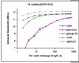
One of the features of our GBN reliable layer is the support of piggyback acknowledgement scheme. Since the communication schedule of pairwise exchange involves only a single partner in each round, we can apply optimization techniques such as piggyback and delay acknowledgement to reduce the control traffics. Based on this optimized implementation, we see that the pairwise exchange algorithm works faster than the shift exchange algorithm in all cases, although they both have the same communication complexity. This is a typical example on the tradeoff between simplicity against accuracy on the performance analysis issue. In Section 5.3, all analyses on different communication schemes are based on the assumption of the send-and-forget nature [8] of asynchronous communication. However, as the underlying network is unreliable, we have to build a reliable protocol layer to accomplish reliability. This protocol layer would induce some control traffics that inevitably interferes with the normal data flows.

Figure: Achievable bandwidth per node for different algorithms as compared to the optimal prediction

[Connected by the IBM 8275-326] [Connected by the IBM 8275-416]

Figure 5.3 shows the achieved bandwidth of these algorithms for p=16 against different message sizes (k) range from 2 to 768 (data packets) on the two switches. Achieved bandwidth is a metric which measures the efficiency of the algorithm in utilizing the network. This is calculated by dividing the total data message sizes per node with the measured communication time. The results show that synchronous shuffle exchange performs the best with the achieved bandwidth for each node reaches 11.82 MB/s (on IBM 8275-416), which is 97% of the available bandwidth. While the measured best achievement for shift exchange is 11.25 MB/s on IBM 8275-416, pairwise exchange is 11.6 MB/s on IBM 8275-326 and group shuffle is 11.8 MB/s on IBM 8275-416 respectively.

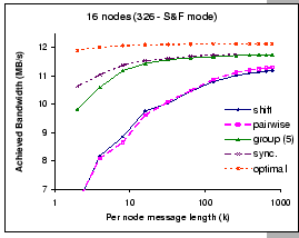
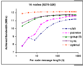
For very long messages (large k), both shift exchange and pairwise exchange are catching up with the performance of the synchronous shuffle exchange algorithm. However, for exchanging small to medium size messages in shift exchange and pairwise exchange, the waiting time incurred by each communication round cannot be masked away and results in poor performance. For example, at k=4, we observed that the achieved bandwidth of the pairwise exchange is 72% of the optimal performance, while the achieved bandwidth of the synchronous shuffle exchange reaches 92%. Furthermore, it is interested to see that the optimization techniques adopted in the pairwise exchange algorithm looks more promising on the virtual cut-through switch (IBM 8275-326) then on the store-and-forward switch (IBM 8275-416). We have repeated the same experiment on IBM 8275-326 with the cut-through mode being switched off, and we experienced the same performance pattern as reported on the IBM 8275-416 switch (in Figure 5.4).

Figure 5.4: Achieved bandwidth on IBM 8275-326 with store-and-forward switching

On the other hand, the synchronous shuffle and the group shuffle exchanges perform much better even up to k=100. The synchronous shuffle scheme logically schedules all communications at the packet level in a pattern that avoids node and switch contentions. As waiting time is removed, the network links are better utilized, and we can exchange all the messages by minimal time, hence, achieved better performance. Theoretically, at the same instant, all packets arrived to different input ports are destined to different output ports according to our contention-free schedule. Therefore, this schedule should operate efficiently on any non-blocking network.

In reality, no global clock is implemented and the operations are not lock-step synchronized. The shuffle pattern of the synchronous exchange could induce head-of-line blocking on the input-buffered switch. The group shuffle exchange algorithm limits the degree of fan out and introduces minimal waiting time during the communication. As shown in Figure 5.3, it performs almost as good as the synchronous shuffle exchange algorithm even at small k.

5.4.2 Effects on Group Size $\omega$

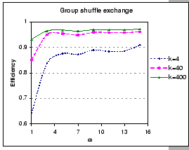
In Figure 5.5 we compare the efficiency of the group shuffle exchange algorithms with respect to different group size $\omega$ for p=16 on various per node message length k=4, 40, 400. Technical speaking, with $\omega =1$, the synchronous shuffle exchange reduces to the pairwise exchange, while $\omega =15$ corresponds to the synchronous shuffle exchange. Clearly, this figure shows that synchronous shuffle exchange always performs the best in all aspects. The group shuffle exchange performs considerably well even under small $\omega$ for medium to large messages as compares to pairwise exchange.

Figure 5.5: The efficiency of the group shuffle exchange algorithm as a function of group size $\omega$ for various message size k on 16 nodes over the IBM 8275-326.

As the performance of the synchronous shuffle algorithm deteriorates under heavy traffic when p is large (will be discussed in the next subsection), the group shuffle algorithm becomes an alternative in achieving higher performance.

5.4.3 Scalability on Problem Size k

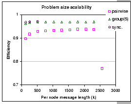
We compare the scalability of these algorithms when operated on the input-buffered switch (IBM 8275-326) with p=16 and $\omega$=5 while varying the problem size k. This test reveals the effect of HOL problem while transmitting long messages. Figure 5.6 shows the results of this experiment. Clearly, we see that synchronous shuffle exchange achieves the best performance, however, the performance degraded significantly after $k>512$ (out of the range shown in the graph), which corresponds to the transmission of total message length 11 MB per node. The performance of group shuffle exchange is only slightly worse than the synchronous shuffle exchange, and it continues to operate at high efficiency until $k>2304$ (around 49 MB per node). Lastly, we observe that the pairwise exchange continues to work for very large message length (around 54 MB per node), but the performance drops dramatically as the required total messaging buffer size is approaching the machine limit, which is around 128MB. In summary, the group shuffle exchange algorithm shows its robustness in dealing with the HOL problem and can retain good performance for very large message sizes.

Figure 5.6: Comparison of the problem size scalability on the input-buffered switch (IBM 8275-326) for p=16

5.4.4 Comparing Switching Mechanisms

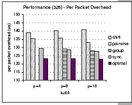
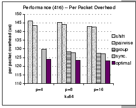
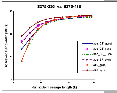
Since the complete exchange operation induces heavy network loading that stresses on the communication network severely, it could be used as a tool to evaluate the relative performance of different hardware components. Figure 5.7 shows the achieved bandwidth of the group shuffle scheme and synchronous shuffle scheme for p=16 on our two switches. Generally, both switches have the similar performance for long messages, so not much difference between the cut-through or store-and-forward modes. However, on short message exchanges, if we cannot fully utilize the network, we cannot effectively mask away the higher latency of store-and-forward switching. This is being reflected by the slower performance of the group shuffle scheme on both switches when they are working in store-and-forward mode. Furthermore, we observe that the switch internal buffering mechanism does affect the overall performance. The performance of the synchronous shuffle exchange algorithm on the output-buffered switch (IBM 8275-416) is always better than the same algorithm on the input buffered switch (IBM 8275-326) with both packet forwarding modes.

Figure: Comparison of performance between a virtual cut-through switch (IBM 8275-326) and a store-and-forward switch (IBM 8275-416) on the synchronous shuffle and group shuffle algorithms

5.4.5 Comparison with MPICH

In Chapter 4, we observe that under heavy congestion loss, our reliable protocol may not be working efficiently due to its simplicity. For examples, we are using static window size and retransmission timer, while the sophisticated TCP/IP protocol adopts many features [93] in handling the congestion issue. Since congestion loss occurs mainly at high network load, one would think of switching back to the traditional protocol stack while we are having intensive communication scheme, such as the complete exchange operation.

Figure 5.8: Comparing the performance of the synchronous shuffle complete exchange algorithm with two MPICH implementations

Our objective of devising efficient communication schemes atop of lightweight messaging system is to support high-level programming model such as MPI. Therefore, we have a direct comparison of our DP implementation of synchronous shuffle exchange algorithm against the MPICH [68] implementation of the complete exchange operations. The results are shown in Figure 5.8. There are two complete exchange MPICH implementations in this graph. The curve labeled as ``MPICH'' represents the original implementation found in the MPICH package, while the curve labeled as ``pairwise-MPI'' represents our implementation of the generalized pairwise exchange algorithm with the MPI_sendrecv() communication primitive.

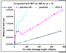
First, we clearly see that the original implementation of the MPI_Alltoall() function by MPICH performs extremely inefficient. This is because their implementation is based on simple non-blocking MPI_Isend() and MPI_Irecv() functions, which are issued in an uncoordinated manner. Therefore, it would subject to both node and switch contention as well as the high overhead problem that inherits from the TCP protocol stack. To avoid the node and switch contention, the ``pairwise-MPI'' carefully coordinates the communications, and achieves considerable improvement. However, our DP implementation of synchronous shuffle exchange even outperforms the ``pairwise-MPI'' implementation significantly. This shows that the traditional protocol stack has severe limitation on achieving high-speed communication. In other words, it is inadvisable to drive the high-performance communication network with the conventional communication protocols.